5/4/15: Angular Acceleration Lab 16

Purpose: Apply a known torque to an object that can rotate and measure the angular acceleration. Use the measured angular acceleration to calculate an experimental moment of inertia and compare it to a theoretical value of moment of inertia.

Procedure / Set Up:

The set up consists of 2 stacked disks that are placed adjacent to a Pasco rotational sensor. On top of the disks is a torque pulley with a string wrapped around it. The string is attached to a hanging mass which goes over another pulley at the edge of the apparatus. When the compressed air is turned on, the disks rotate independently and the hanging mass moves up and down.

The experiment is broken up into two parts

Part 1: We will be performing 6 different experiments/ trials and measuring the angular acceleration of each one as well looking at how various changes in the experiment effect the angular acceleration of our system. In addition we will use one of our trials and look at v (hanging mass) vs. ω (disk) and a (hanging mass) vs. α (disk)






Before beginning the actual experiment, a few measurements needed to be made using a pair of calipers and an electronic balance. 

To begin, clean all the disks with alcohol before using the apparatus. Plug in the power supply to the apparatus and connect it to Logger Pro. Be sure to choose the rotary sensor and set the sensor settings to 200 counts per rotation, as there are 200 marks on the top disk. The hose clamp on the bottom of the apparatus should be open in order for the disks to rotate independently of each other. Turn on the compressed air, but just enough to keep thing smooth and with the string wrapped around the torque pulley and the hanging mass is at its highest point, hit collect on Logger Pro. Taking the slope of the graph of angular velocity vs. time can be done to determine the angular acceleration of the system. This will be done for all 6 trials.

Important Note:

We take an average angular acceleration from the up and down motion because when the mass descends, there is frictional torque slowing down the disk and torque from the string speeding up the disk. When the mass ascends, there is frictional torque from the disks and frictional torque from the string slowing down the disk.

Below is an image better explaining this complication.  

 

After completing each trial, there should be 6 different recorded angular acceleration values. Below are two examples of our data analysis for part 1. Each trial looks pretty much the same. 

Effects to look at by various changes in the experiment for each trial.

Trial 1, 2, and 3: Effects of changing the hanging mass

Trial 1 and 4: Effects of changing the radius at which the hanging mass exerts a torque

Trial 4, 5, and 6: Effects of changing the rotating mass (disks).

Trial 2: 

2 x hanging mass

Small torque pulley

Top Steel disk

Taking the slope of the angular velocity vs. time will yield the angular acceleration. α = 1.259 rad/s^2 for this trail.

Trial 5:

hanging mass only

Large torque pulley

Top aluminum disk

Again, taking the slope of the angular velocity vs. time graph gives the angular acceleration. α = 3.444 rad/s^2

Compiled data shown below:

For experiment 6 we added a motion sensor to our set up to compare v (hanging mass) vs. ω (disk) and a (hanging mass) vs. α (disk)

This graph represents v (hanging mass) vs time and by taking the slope of the up and down motion, we were able to get a (hanging mass).

 This graph represents ω (disk) vs. time and again taking the slope will give us α (disk).

Below is the graph of v (hanging mass) vs time. By taking the mean of the up and down values, we can get v average.

Below is a graph of ω (disk) vs. time and again taking the mean of the up and down values, we can get ω average.

Using the same method in determining the average acceleration of our system, we can get v (hanging mass) vs. ω (disk) and a (hanging mass) vs. α (disk).

Conclusion Part 1: By various changes in the configuration of the apparatus, we noticed that the greater the hanging mass the greater the angular acceleration. Experiment 2 had 50 grams of hanging mass with an angular acceleration of 1.259 rad/s^2 and experiment 1 had 25 grams of hanging mass with an angular acceleration of 0.6274 rad/s^2. Another observation was that as the radius of the torque pulley is increased, the larger the value of angular acceleration would be. Experiment 1 had a smaller torque pulley radius and an angular acceleration of 0.6274 rad/s^2, while experiment 4 had the larger radius with angular acceleration of 1.217 rad/s^2. One last observation made was that the more massive the rotating disks, the slower the angular acceleration was. Experiment 5 used an aluminum disk and generated an angular acceleration of 3.444 rad/s^2 while experiment 6 used a steel disk and generated an angular acceleration of 0.641 rad/s^2.

Part 2: Use our data from part 1 to calculate an experimental moment of inertia and compare it to a theoretical moment of inertia.

Because our system is not completely frictionless, α isn't the same when the mass ascends and descends. Below is a simple derivation of how we will calculate an experimental moment of inertia. The theoretical moment of inertia is simply the moment of inertia of a disk. 

Below is our experimental moments of inertia vs. theoretical moments of inertia. 

Conclusion part 2: As you can see, our experimental and theoretical values do not match at all. There is a 78% error from experiment 1 and  similarly for experiment 2. This is an extremely high error. 

Overall Conclusion:

In part 1, we measured the angular acceleration of a system by applying a known torque. We looked at the effects on α by varying the configuration and compared them to each other. We set up a motion sensor to look at v (hanging mass) vs. ω (disk) and a (hanging mass) vs. α (disk). In part 2, we used our values from part 1 to calculate an experimental moment of inertia and compare it to a theoretical value of moment of inertia. As observed, our values did not compare well, all the data from part 1 seemed correct.

Error in our values could have been due to not setting the rotary sensor to read 200 marks. At one point in our trials, we realized we had the wrong disk on top and had to restart, which could have possibly caused us to forget to change the sensor settings back to 200 marks. Another source of error could have been from improperly handling the disks. We made sure to clean them with alcohol, but as we were swapping them we put finger prints all over to bottom and top of the disks. Over all, the final results of our experiment did not come out as precise as we had hoped. 

5/13/15: Moment of Inertia of a Uniform Triangle Lab 17

Purpose: Determine the moment of inertia of a right triangular thin plate around its center of mass, for two perpendicular orientations of the triangle. We will compare an experimental value of moment of inertia to a theoretical value of moment of inertia. 

Procedure / Set Up:

The set up consists of 2 stacked disks that are placed adjacent to a Pasco rotational sensor. On top of the disks is a torque pulley with a string wrapped around it as well as triangle mounted on a holder. The string is attached to a hanging mass which goes over another pulley at the edge of the apparatus. When the compressed air is turned on, the disks rotate independently and the hanging mass moves up and down.

Approach - Theory:

We want to calculate the moment of inertia about the center of mass of a thin triangular plate, but because the limits of integration are simpler if we calculate the moment of inertia around a vertical end of the triangle, we can calculate that moment of inertia and use the parallel axis theorem to then get the moment of inertia around the center of mass.

The parallel axis-theorem is give by:

Since we will be calculating the moment of inertia of the triangular plate in two different orientations, upright and sideways, the tension in the string will exert a torque on the pulley-disk combination and by measuring the angular acceleration of the system we can determine the moment of inertia of the system. We will accomplish this by measuring α of the (disk + holder), α of (disk + holder + triangle), determining I of (disk + holder), I of (disk + holder + triangle), and the difference between the two moments of inertia will give us the moment of inertia of the triangle. These will be our experimental values for I. In total, we will compare four different values.  

Before beginning the experiment, we derived and expression for (I around cm), which will be our theoretical value. By using the parallel axis theorem, I = 1/18 ML^2
This equation for I will be the same for both the upright and sideways orientations. 
where M = 0.455 g, L = 0.0983 m (upright), L = 0.1493 m (sideways)

Because of frictional torque in the system, the rotating disk isn't truly frictionless and there is mass is the frictionless pulley. We derived an expression for the the moment of inertia of the system following this approach back in the angular acceleration lab. The derivation is shown below. The boxed equation on the bottom left is the one to notice.

Now we can measure α of the (disk + holder), α of (disk + holder + triangle), and determine I of (disk + holder) and I of (disk + holder + triangle).

Upright Triangle:

How the setup should look at this point for α of the (disk + holder).

α of the (disk + holder) was determined by allowing the mass to rise up and down while Logger Pro generated the angular velocity graph.The slope of ω vs. t would give us the α. 

An average was taken of α up and α down in order to find α of the system. I of (disk + holder) was then calculated as shown below. I = 9.237 x 10^-4 kg*m^2

Using the same logic as above, I of (disk + holder + triangle) was calculated as shown below.

Graph of ω vs. t for (disk + holder + triangle) to find α

Using α to find I (disk + holder + triangle) calculation.

The difference between the two moments of inertia will give us the experimental moment of inertia of the upright triangle. I = 2.482 x 10^-4 kg*m^2. Using the theoretical derivation I = 1/18 ML^2, we concluded I = 2.44 x 10^-4 kg*m^2. Comparing these two values, we get a percent error of 1.721 %.

Sideways triangle: 

How to set up should look:

Once again α of the (disk + holder) was determined by allowing the mass to rise up and down while Logger Pro generated the angular velocity graph.The slope of ω vs. t would give us the α. I (disk + holder) is the same value as was in the upright triangle I = 9.237 x 10^-4 kg*m^2.

The same logic was applied as from the upright triangle. α of the system (disk + holder + triangle) was determined by taking an average of α up and α down from the slope of the ω vs. t graph.

The difference of I of (disk + holder) and I of (disk + holder + triangle) would give us the experimental value of I for the sideways triangle. Below are the calculations.

By comparing the experimental value I = 5.587 x 10^-4 kg*m^2 and the theoretical value I = 5.634 x 10^-4 kg*m^2, we se we have a percent error of  0.834 %.

Conclusion: 

Our goal was to determine the moment of inertia of a triangular plate in two different orientations. We were able to achieve this by using the parallel axis theorem. We derived an expression for the moment of inertia, measured α of the system, calculated I of the system, and lastly compared an experimental value to a theoretical value. Our percent error for both orientations was relatively low, so it is safe to say the experiment was a success. An error we encountered at first was that our percent error for the sideways triangle was relatively high, but it was easily fixed by remeasuring the length of one of the sides of our triangle. 

5/11/15: Moment of Inertia and Frictional Torque Lab 18

Purpose: Use Newtons second law of rotation to determine the time it takes for a cart to travel down an incline while attached to a large metal disk by a string.

Procedure / Set up:

The apparatus consists of a large disk on a central shaft and at the center of the disk are smaller cylindrical disks that serve as an axis of rotation.

As the cart is traveling down the incline, the disk exerts a frictional torque opposite the carts direction of motion. So before actually predicting the time it would take for the cart to travel 1m, we need to measure the frictional torque exerted by the apparatus. To accomplish this, we will need to determine the total moment of inertia and the angular acceleration of the apparatus. (T frictional = Iα)

Determining the total moment of inertia:

Measure and record the dimensions of the larger central disk and the two smaller side cylindrical disks. These values will be used to determine the volume of each piece. The smaller disks are labeled (1) and (3) and the larger disk is labeled (2). 

The ratio of the volume for a piece divided by the total volume of the apparatus will give us the percentage of mass for that piece. For example if 86 % of the total mass of the apparatus belongs to the central disk, then we can take that value and multiply it by the total mass of the apparatus to find the mass of just that central disk. The total moment of inertia is the sum of the moment of inertia of the central disk plus the two moments of inertia for the smaller cylindrical disks. 

Determining the angular acceleration:

We set up a camera so that its lens lines up directly with the apparatus' axis of rotation.

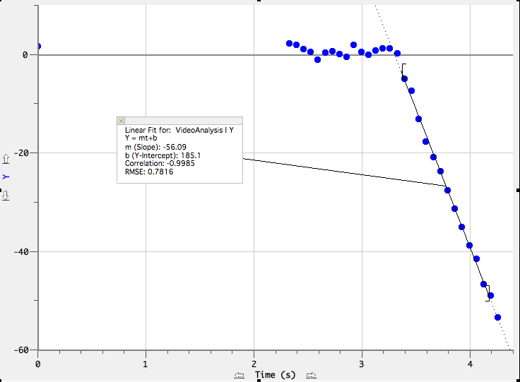
Our plan was to capture the disk as it rotates and use the Logger Pro video capture software to find the angular deceleration of the disk. To do this, we marked a point on the disk, recored the disk while it spun, and analyzed the video. During the analyzation process we plotted a point every time our marked spot on the disk went through one revolution or 2π radians. We did this for 15 revolutions or 30π radians. By plotting a point every revolution, Logger Pro would automatically create a column for the time is took to complete that revolution. We next created a column titled theta (ø). This column consisted of the number of radians traveled by the point every 2π revolutions/increments. We next plotted a graph of ø vs. t to find the angular acceleration of the disk.

The equation ø = At^2 + Bt + C is very similar ø = 1/2αt^2 + ωt, Therefore 2A is our actual value for angular acceleration, which equates to -1.075 rad/s.

Because T = Iα, we can now say our value for frictional torque is -0.02265 N*m.

Determining the time it takes the cart to travel down the incline:

The set up consists of the apparatus along with a track at the edge of the table, with the track inclined around 44º. A string is tied around the smaller cylindrical disk and then tied to a cart. The track is positioned so that it is parallel to the string.

Before running the experiment we are asked to predict the time it will take the cart to travel 1m. By drawing a free body diagram of the situation and using Newtons second law of rotation and along with kinematics, the time we determined it would take the cart to travel 1m was 9.42 seconds. 

With our predicted value at hand we performed four trials and recored the times for each.

T1: 9.38 s

T2: 9.50 s

T3: 9.44 s

T4: 9.41 s

These values averaged to 9.432 seconds, which gave us a percent error of 0.127 %

Conclusion:

In this lab, our main goal was to determine the time it would take a cart to travel down an incline when attached to cylindrical rotating disk. We were able to find this value using concepts from Newtons second law of rotation, moment of inertia, kinematics, and rotational kinematics. The main steps were calculating the total moment of inertia of the apparatus, measuring the angular deceleration of the apparatus with Logger Pro video capture, and deriving an equation that would express the linear acceleration of the cart enabling us to find the time. The more difficult part of the lab was coming up with a method for finding the angular deceleration of the apparatus. Although our final error was relatively small, error could have been introduced from uncertainty in measurements or from unaccounted friction from the track. 

4/27/15: Ballistic Pendulum

Purpose: Determine the velocity of a small metal ball fired from a spring loaded gun using conservation of momentum and conservation of energy.

Procedure / Set Up:

A small metal ball will be initially at rest in spring loaded gun. Once fired, it will collide with a pendulum/casing that is initially at rest and then swing through some angle ø. The angle will be recorded with a thin metal rod that swings up immediately after the ball collides with the pendulum. 

Once the ball was fired, the values needed to determine the initial velocity of the ball were

Mass of ball (m): 0.00763 kg       dm = +/- 0.0001kg
Mass of pendulum (M): 0.0809 kg       dM =  +/- 0.00001 kg
Length of string (L): 0.197 m       dL = +/- .001 m
Angle (ø): 17.0º       dθ = +/- 0.00873 rad

By first using conservation of momentum, we derived an equation for the initial velocity of the ball. We next used conservation of energy to derive an equation for the final velocity of the ball. Next we substituted the final velocity from our conservation of energy equation into the final velocity of our conservation of momentum equation to find a final equation that would allow us to determine the initial velocity of the metal ball. 

We can now plug in our measured values into the derived equation and solve for v0, which equaled 4.765 m/s.

Because there is always some error when making measurements, our initial velocity was not 100% accurate. We therefore needed to calculate the uncertainty in V0.

Below is our derived uncertainty calculation for dv.
dv = 0.02089 m/s

 

The initial velocity at which the metal ball exited the spring gun was 4.765 +/- 0.2089 m/s

 

Conclusion:

 

We were able to calculate the initial velocity of a metal ball fired from a spring loaded gun using conservation of momentum and conservation of energy. Even though we calculated the error in our measurements, there is still other errors to factor in such as the friction from the ball on the spring gun. In general, we derived an equation to find a reasonable speed and reasonable uncertainty for the initial velocity of the metal ball.



4/22/15: Collisions In Two Dimensions Lab 15

Purpose: Determine if momentum and energy are conserved by looking at a two-dimensional collision.

Experiment / Procedure: 

This lab consisted of setting up two elastic collisions using a steel ball paired with another steel ball and a steel ball paired with an aluminum ball. We used a smooth glass table with a camera mounted on it to give a birds eye view of each collision. The camera captured the data needed to determine if momentum and energy were conserved.

Part 1: Steel Ball and Steel Ball Collision

We used the video capture software on logger pro to plot the position of each ball before, during, and after the collision. To actually do the calculations, all we needed was the mass of the balls and the graphs generated by Logger Pro. M steel ball = 66.8 g

As the points are being plotted for each ball, Logger pro will generate graphs for the x and y motion of each. The graphs can be used to determine the initial and final x and y components of velocity for each ball.

Below is the position vs time graph of the ball that is initially rolling and by taking the slope of the graph, the initial velocity can be determined. The initial speed of the rolling ball before the collision Vo1 = 188.3 and the final velocity of the x component V1f,x = 104.5

  

Next, we can look at the y components of velocity for the ball that is initially rolling

Below shows the y component of the final velocity. V1f,y = 56.09 and the initial velocity of the first rolling ball in the y direction is 0. Taking the slope of the position vs. time graph will yield the velocity.

Next we examined the ball that was initially at rest. The initial x and y components will both be 0. (Ball is initially at rest). Again, by taking the slope of the position vs. time graph will give the velocity. 

The final y component of velocity V2f,y = 58.98

Below shows the the final x component of velocity V2f,x = 75.85

Now that we have all of our required values, we can see if momentum and energy were conserved. The equations necessary for this step are shown below as well as the actual calculations. 

Conservation of momentum and conservation of energy. 

Calculations

Below, the finals values are not exact, but we can see that momentum in the x and y directions should be conserved. 

Below shows that energy was lost. It could have been lost due to heat and sound when the collision occurred.

Part 2: Steel Ball and Marble Collision

The same set up is used as in part 1 except we will be replacing one of the steel balls with a marble. We plotted points again and analyzed the motion of our graphs, took the slope to determine the velocity, and used the necessary equations to see if momentum and energy were conserved. Mass of marble = 20.7 g and mass of steel ball = 66.8 g

Below are the calculations. The graphs are almost identical to the ones from part 1, only the slopes have changed. Note that M = steel ball and m = marble

Conservation of Momentum

Again it was observed that momentum should be conserved in both the x and y directions. 

Conservation of Energy

Below the calculations show that some energy was lost and again most likely due to heat and sound. 

Conclusion: Our main objective was to see if momentum and energy were conserved for two elastic collisions. Once we had determined the velocities of each ball in the x and y directions and substituting those values into the proper equations, we were able to see that in both situations, momentum was conserved, but energy was not. In a perfectly elastic collision, no kinetic energy should be lost. In part 1, the difference in energy is somewhat significant, and in part 2 the final and initial kinetic energies are a little bit closer. Again, the energy loss is most likely due to heat, sound, or improper analysis of the video. Another source of error could have been from not choosing the exact same point on the ball when we plotted it frame by frame, as it should have been done from the center of the ball. 

4/16/15: Impulse - Momentum Lab 14

Purpose: The impulse-momentum theorem states that the change in momentum for a moving cart is equal the net impulse acting on the cart (∆p = J). Our job is to test this idea by performing three experiments.

Expt 1: Observing Collision Forces That Change With Time

A dynamics cart with its spring plunger extended is clamped to the table using a rod and c-clamp. On the other end of the track is a force sensor mounted to another dynamics cart with a rubber stopper in place of the force sensors hook. Be sure to level the plunger with the rubber stopper so they can correctly collide with each other. 







For the first part of this experiment, we will be measuring a non-constant force over a time interval ∆t. In order to verify the impulse-momentum theorem (∆p = ∫ Fdt), we will need to measure the mass of the cart and use logger pro to generate a force vs. time graph and a velocity vs. time graph, as we will be needing the velocity of the cart right before and after the collision. Once the apparatus has been set up, open the file called Impulse and Momentum (L08A2-2), calibrate the force sensor and re-attach it the moving dynamics cart. Once ready, zero the force probe and hit collect to begin graphing. Give the cart a push toward the stationary cart and let it collide with the plunger and bounce back. Once logger pro has generated a force vs. time graph, open up an axis that shows velocity vs. time.

By analyzing the graph of force vs. time using an integral fit, the impulse imparted (∫ Fdt) on the cart was 0.7481 N*s.

Using the final and initial velocity values of the cart as well as the mass, the change in momentum (∆p) can be calculated. ∆p = 0.754 N*s

Since J = 0.7481 N*s and ∆p = 0.754 N*s, we can say the impulse does closely equal the change in momentum.

Expt 2: A Larger Momentum Change

Using the same set up an in part 1, we added mass to the cart and repeated the experiment to see if the impulse-momentum theorem still held true.

Again by analyzing the force vs. time graph using an integral fit, we can obtain the impulse imparted on the cart which equaled 1.248 N*s

Using the final and initial velocity values of the cart as well as the new mass, the change in momentum (∆p) can be calculated. ∆p = 1.298 N*s

Again J = 1.248 N*s and ∆p = 1.298 N*s, we can say the impulse does closely equal the change in momentum.

Expt 3: Impulse - Momentum Theorem in an Inelastic Collision

In this experiment we used the same set ups as in part 1 and 2, except this time a wooden block with a blob of clay will be in place of the stationary dynamics cart. A nail will be attached to the rubber stopper on the force sensor hook as well. We kept the mass of the cart the same as in part 2 (1.092 kg). 

We hit collect on logger pro and gave the cart a push towards the wooden wall and analyzed a force vs. time and velocity vs. time graph.

Using an integral fit, we measured the impulse to be J = 0.4276 N*s

Since the final velocity of the cart is 0 m/s we analyzed our velocity vs. time graph and found the initial velocity of the cart to be 0.3859 m/s. Our change in momentum ∆p = 0.4225 N*s

Because J = 0.4276 N*s and ∆p = 0.4225 N*s, we can verify the impulse-momentum theorem once again hold true for this experiment.

Conclusion:

For this lab, we wanted to verify the impulse-momentum theorem (∆p = J). We were able to do this by performing three different experiments: two elastic collisions, and one in-elastic collision using dynamics carts. In all three experiments, the impulse imparted on the cart nearly equaled the change in momentum of the cart. If the experiment was perfect, the two values would be exactly the same. Some error within the experiment could have been due some slight friction on the track even though its supposed to mimic a frictionless surface. Another source of error is from the bumper on the stationary dynamics cart. In a perfectly elastic collision, the cart would recoil with exactly the same momentum it had before the collision. Over all, we can conclude the theorem holds true.