3/25/15: Centripetal Acceleration vs. Angular Frequency Lab 8

Purpose: Use an accelerometer to determine the relationship between centripetal acceleration and angular speed.

Materials: An accelerometer mounted onto a disk and a scooter wheel used to revolve the disk such that the accelerometer passes through a photogate positioned on a pole.

Procedure: The disk was spun using the scooter wheel and the amount of time to complete 10 rotations was recorded at six different speeds. The distance of the accelerometer from the center of the rotating disk was also measured as well as the accelerometer reading corresponding to each speed.

We recorded and were able to generate six different speeds using six different voltages: 4.8, 6.2, 7.8, 8.8, 10.8, and 12.6. a is the centripetal acceleration, t(0) represents the time the first rotation occurred through the photogate and t(10) represents the time at which the 10th rotation occurred. 

Centripetal acceleration is calculated using the formula a=v^2/r, where v=rω (How we relate linear speed to angular speed). Therefore, a=rω^2 and by rearraging to solve for r, we can find the radius. An acceptable value would be 13.8 - 14.0 cm. 

ω = 2π rad / time for 1 rotation.

After running and recording six different speeds, we input our values into logger pro to generate a graph of acceleration vs. angular speed^2 and compared our slope with the acceptable value. 

the last two columns were calculated columns. 

ω was calculated using 10 rotations from t0 to t10

Once we input an equation into the calculated columns, we generated our plot. Using a best fit line, the value for our radius was .1371 m or 13.71 cm. 

Conclusion: The slope of the graph above displays the radius of the disk 13.71 cm. As the theory predicts, if we increased or decreased the angular speed or acceleration, the radius would do the same. Some sources of error could have been friction from the wheel on the disk or the tape slightly grazing the photogate. Another source of error to note is that t0 does not always begin exactly when time is 0 seconds. This means the tapes initial position was slightly different for each trial. 

3/23/15: Trajectories Lab 5

Purpose: To use our knowledge of projectile motion in order to predict the distance a ball will travel before impacting and inclined board.

Materials:

1. aluminum v-channel
2. steel ball
3. board
4. ring stand with clamp
5. carbon paper
6. tape
7. ruler
8. plumb bob

A complete set up of the apparatus

Procedure Part 1: Once the apparatus has been set up, we launched the steel ball from an identifiable point on the v-channel to see where it would land. We placed the carbon paper at the impact point on the floor and launched the ball five more times to get a more accurate distance of how far out from the tables edge the ball landed. We hung a plumb bob as well to get even more accuracy. After observing the marks on the carbon paper we used a meter stick to measure the distance from the edge of the table to the impact point. 

The measured horizontal distance was 0.734 meters. We were asked to determine the launch speed of the ball, so we needed the vertical height as well, which was 0.874 meters.

Using kinematics in two dimensions, we calculated the time the ball was in the air using the vertical height and gravity. Once we had the time, we were able to determine the speed.

The time in the air is for both x and y components, but the initial velocity is only in the x direction.   





Procedure Part 2: After calculating the launch speed, we had to imagine attaching an inclined board at the edge of the table and when launched from the same position, the ball will strike the board a distance d along the board.

The horizontal distance was 0.835 meters and the vertical distance was the same as in part 1.
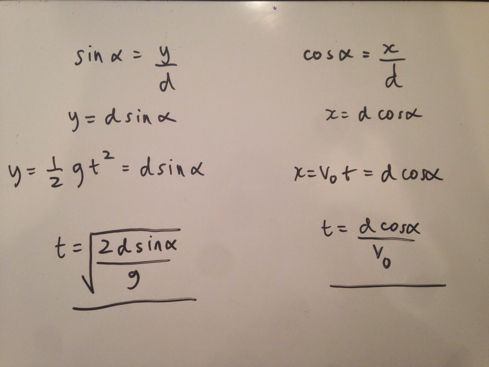
We measured the angle α to be 46.3º using tan^-1(y/x)







Given that we know the values of v0 and α, we derived an expression that would allow us to determine d along the board. 

Our experimental value of d was 0.947 meters. 

Once we determined d we set up the apparatus again, but with the board held in place by a weight and tape. 

We then placed the carbon paper along the board a distance d, based on our experimental value and launched the ball five more times from the same initial point as in part 1. 

The mark inside the red square is the impact point along the board. We next calculated the uncertainty in our experimental value of d.

In our derived equation for d, we needed an expression for v0 that represented a function of x and y. we started with the equation v=x/t and used the x and y components of the projectile to create an expression for v0 that we could plug into our propagated uncertainty formula. 

Our uncertainty for measuring the distance in the x and y direction was +/- 0.01 m and the uncertainty for the angle was +/- 0.0174 radians.

Above is the experimental calculations for d. 

Conclusion:

The equation used in calculating percent error

Our calculations showed that d = 0.936 m +/- 0.125 m. Our measured theoretical value was 0.890m. This yields a % error of 5.17%, which shows our experimental value compared well to our theoretical value. Possible sources of error could have been accidental moving of the board or v-channel. The v-channel was constantly being readjusted due to slipping. We could have easily avoided this by using tape. 

3/18/15: Modeling Friction Forces Lab 7

Purpose: To apply Newton's laws throughout five different experiments in order to determine the coefficients of kinetic and static friction.

Part 1 Static Friction:

We will be determining the coefficient of static friction using a pulley, wooden block, and cup. Below is an image of how to set up the experiment.

A wooden block with the felt-side placed on the table and a string attached to the block. A cup is attached to the string which hangs over the table by a pulley.

The procedure goes as follows:

1. Weigh a wooden block and record the mass. The system should be at rest before beginning. 
2. Carefully add water to the cup until the block begins to move. Record the mass of the cup.
3. Record the mass of another wooden block and place it on top of the existing block. Record the total mass of the blocks.
4. Carefully add water again to cup just until the blocks move. Record the mass of the cup with water.
5. Repeat this process until you have four blocks stacked on top of one another
6. By the end, a total of four different values of mass for the blocks and four different values of mass for the cups with water should be recorded.

Below is the collected data and free body diagram of the set up

We will input this data in to logger pro to determine the maximum coefficient of static friction.

Below is a data table consisting of our values input into logger pro

The force of friction should equal M Water + cup, which is the mass of the cup with water. We made sure to convert grams to kilograms. 

To determine the coefficient of static friction we plotted a friction force (N) vs. normal force (N) graph. The slope of the graph is our coefficient which was 0.3093.

Part 2 Kinetic Friction:

We will be measuring the coefficient of kinetic friction using a force sensor, wooden blocks, and string. Before beginning we made sure to calibrate the sensor with using a 500 g hanging mass. Using the same wooden blocks as before, we pulled the block across the table at constant speed, recorded the data in logger pro, and repeated this process until we generated four different graphs. By pulling the blocks at constant speed, the force of kinetic friction will equal the force of the pull. 

Once all four graphs have been created in logger pro, we determined the mean force exerted on each stack of blocks and generated another graph to find the coefficient of kinetic friction.

The mean value is the force exerted on each block. These values were the graphed and the slope of the graph represented to coefficient of kinetic friction. 

Friction (N) vs. Normal Force (N)

Our value was 0.2531. This makes sense seeing that the coefficient of kinetic friction should be smaller than the coefficient of static friction.

Part 3 Static Friction From A Sloped Surface: 

Again we will be measuring the coefficient of static friction, but this time using only a track and wooden block. We began by placing the block on a horizontal track, slowly raising one end of the track until the block started to slip. We then measured and recorded the angle the track made with the horizontal.

 

We were able to determine the coefficient of static friction by drawing a free body diagram and summing up the forces in the x and y direction. The force of static friction is equal to mgsinø because there is no acceleration in the x direction. We figured out µs is simply equal to tanø. 


Part 4 Kinetic Friction From Sliding A Block Down an Incline:

We will now be measuring the coefficient of kinetic friction. We set up a motion detecter at the top of a horizontal track steep enough so that a block will accelerate down the incline. We measured the angle of the incline and used a velocity vs. time graph to find the acceleration of the block. With this information we can use a free body diagram to again find µk. 

Set up of experiment

We used logger pro to collect a position vs time and velocity vs time graph. The slope of the velocity vs time graph is the acceleration of the block.

A free body diagram drawing of the set up and sum of all the forces leading to µk.

Part 5 Prediction the Acceleration of a Two-Mass System:

This last experiment we will take our coefficient of static friction and use it to derive an expression for what the acceleration of the block would be if we used a hanging mass heavy enough to accelerate the system. The set up used is a track, motion sensor, hanging mass, wooden block, pulley, and string. 

Below is a free body diagram and an equation we derived for the acceleration of our system. Based on µk we determined the acceleration to be 2.675 m/s^2.

We next used logger pro to generate a velocity vs. time graph and found the slope from the graph to be 1.137 m/s^2. Our values did not quite match.

Conclusion:

For this experiment, we determined µs and µk for various situations. We saw how pulling a mass at constant speed leads to µk being equal to the force our pull generated. We learned how to calculate µs from something as simple as raising a track and recording the angle it made with the horizontal when the block slipped. To tie it up, we used our value for µk to predict the acceleration of a system.

3/02/15: Non-Constant Acceleration Lab 3

Purpose: Analytically and numerically solve a non-constant acceleration problem. Be able to successfully apply various formulas into an excel spreadsheet, as well as see the logic behind it, that would generate the same answer as when when solving the problem analytically.

Problem: A 5000 kg elephant on frictionless roller skates is going 25 m/s when its gets to the bottom of a hill and arrives on level ground. At that point a rocket mounted on the elephant's back generates a constant 8000 N thrust opposite the elephant's direction of motion. The mass of the rocket changes with time (due to burning the fuel at a rate of 20 kg/s) so that the 

m(t) = 1500 kg - 20 kg/s*t

Find how far the elephant goes before coming to rest. 

A simple drawing of the scenario. As shown in the picture, we are looking for x.

Analytically:

We are given the elephants acceleration as a function of time. Using Newtons second law, F=ma, we can rearrange to find a(t). The net force is (-) because it is in the direction opposite to the elephants motion. The total mass is the mass of the elephant + mass of the rocket. 

We can next integrate a(t) from 0 to t to find ∆v to derive an equation for v(t).

After integrating a(t) to get v(t), we get the equation below. 

Next we integrate v(t) from 0 to t to find ∆x to derive an equation for x(t)

Equation for x(t) below

Before finding how far the elephant goes before coming to rest, we need to find the time when the final speed of the elephant is zero. Solving for t from the equation below leads us to 19.6907 seconds. 

Lastly, we plug t = 19.6907 s into our x(t) expression to yield x=248.7 m. This will be the distance the elephant travels before coming to rest. 

Numerically: 

Solving this problem analytically can be challenging, luckily we can do it with much more ease using excel. 

We need to create columns as shown below.

1. Column A: Time begins at 0, so start by setting time increments by 0.1 seconds (= A3+$B$1)

2. Column B: Since acceleration is not constant, we need to input into B3 (= -400/(325-A3))

3. Column C: a_avg = (a1+a2)/2 we need to enter in C4 (=(B3+B4)/2)

4. Column D: ∆v = a_avg*t we entered in D4 (= C4*$B$1)

5. Column E: v = vf + vo. In E4 input (=E3+D4)

6. Column F: v_avg = (vf + vo)/2 in F4 enter (=(E3+E4)/2)

7. Column G: ∆x = v_avg*t in G4 we entered (=F4*$B$1)

8. Column H: xf = xo + ∆x lastly in H4 to find the final position we entered (=H3+G4)

We can now make our time increments smaller or larger to see if it make any difference in our answer. Below we see that if we used ∆ t = 0.1 seconds, at 19.6 seconds, our final position if 248.69m, which is pretty much exactly as we calculated analytically. 

By making ∆ t = 1 second we still get a very close position as we calculated analytically, but its not exact. 

Conclusions:

We are able to approach this by imagining a plot of a vs. t. If ∆t is small enough, then the curve between t0 and tf is approaching a line and ∆v between t0 and tf is the area under the curve of the a vs. t graph between t0 and t1. 

We now imagine a graph of v vs. t. If ∆t is small enough we can approximate the curve between v0 and v1, v1 and v2 etc. as straight lines.

1.Doing the problem analytically and numerically yielded the same results. Numerically, the accuracy of the answer depended on the value we used for ∆t. If we used 0.1 as ∆t, we get matching numerical and analytical results. If we use 1 second, there is a small difference in the final position. In general the smaller we make ∆t, the more our analytical and numerical results would match.

2.You know the time interval analytically is small enough when the velocity becomes extremely       close to 0. Another aspect to look at is when the difference in the distance values become close to 0   as well. 

3/04/15 Propagated Uncertainty / Unknown Mass Lab 6

Purpose: The objective of part 1 for this lab was to learn how to calculate propagated error in each of our density measurements using calculus and determine if our measurements were within the experimental uncertainty of the accepted values. Part 2 required us to find the mass of an unknown hanging object using tension and angles, and to use the knowledge acquired from part 1 to calculate the uncertainties in our measurements.

Materials:

small aluminum, copper, and iron cylinders.

An electronic balance was used the measure the mass of each aluminum, copper, and iron cylinders

Calipers that allowed us to measure the height and diameter of each cylinder.

Newton spring scales to measure the force of tension created by the hanging mass. And an angle measuring device to measure the angle the string made with the horizontal.









Part 1:

Procedure: Using the electronic balance and calipers, we were able to measure the height, diameter, and mass of each cylinder. By using our values for mass and volume, we calculated the densities of each cylinder as well.

Since our main goal was to calculate propagated error, we needed values for uncertainty in mass, diameter, and height. We then derived an equation for the density of a cylinder and took the derivative with respect to height, mass, and diameter to create an equation for uncertainty in density.

The calculated uncertainty in density for aluminum, copper, and iron

Summary: The accepted values for the density of aluminum, iron, and copper are as follows:
2.7 g/cm^3, 7.874 g/cm^3, and 8.92 g/cm^3. Our experimental values were: 2.9114 +/- .038 g/cm^3, 7.78 +/- .1375 g/cm^3, and 9.187 +/- .181 g/cm^3. 

Part 2

Procedure: A set up was already completed prior to beginning the experiment. We needed to gather measurements for both the spring scale readings and angles the strings made with the horizontal. 

Unknown Mass #7

Unknown Mass #8

A free body diagram and measured values were drawn and gathered as shown. Using Newtons 2nd law an equation was derived using the free body diagram to determine the mass of #8 and #7.

Again as is part 1, we needed values for uncertainty in F1, F2, ɵ1, and ɵ2. We then used our derived equation from Newtons 2nd law and took the derivative with respect to F1, F2, ɵ1, and ɵ2 in order to generate an equation that would give us uncertainty in mass. It was important to note that the uncertainty in F1 and F2 were different for both set ups and to make sure the uncertainty in ɵ1, and ɵ2 were in radians rather than degrees. 

The calculated uncertainty in mass for set up #7 and #8

Summary: In conclusion, the masses of each set up were calculated to be 828.3g (#7) and 918.4g (#8). The uncertainty values were extremely high with #7 being +/- 98.8 g and #8 being +/- 77.6g. This high uncertainty could be due to wrong angle measurements, due to the fact that it was somewhat difficult to measure the angle and not disturb the spring scales and improper spring scale readings. As a group we learned how uncertainty in measurements leads to uncertainty in our final results.