2/25/15: Sparker Free Fall Lab 2

Purpose: The objective of this lab is to verify that a body in free fall will accelerate at a rate of 9.8 m/s^2.

Materials:

The apparatus shown above is a spark generator attached to a 1.5 m column. At the top of the column is a mass held by an electromagnet and when dropped, the spark generator records the fall/position of the mass every 1/60th of a second onto spark sensitive tape. 

Above is the spark sensitive tape secured next to a meter stick. On the tape there will be a series of dots which correspond to the position of the free falling mass.

Procedure: To save materials, a demonstration of how the apparatus works was done and spark tapes were handed out from a previous class that had run the experiment. After the spark tape was secured next to a meter stick, we lined up the 0 cm mark with one of the dots on the tape, set this dot as our origin, and measured the distance of each dot that appeared after. With this data, we used excel to create five different columns in order to generate graphs that would display our values of acceleration based on the marked positions of the spark tape. We then gathered our class data as a whole, and calculated the average acceleration. 

Data Tables/Graphs:

Column A - Time every 1/60th of a second.

Column B - Distance of every dot after the origin in cm. 

Column C - Change in position between each dot ∆x.

Column D - Time for the middle of each 1/60th of a second interval. (A2+1/120)

Column E - Mid interval speed. (∆x/(1/60)

By selecting columns D and E in excel we were able to generate a graph that compared mid-interval speed vs. mid-interval time. This was done by using an XY scatter graph, adding a trendline, and displaying the trendlines equation along with its R^2 value. Based on our results, the slope of the equation showed the acceleration due to gravity was 932.7 cm/s^2 or 9.32 m/s^2. 

Another graph can be generated by selecting columns A and B (Distance vs. Time). By taking the derivative of the equations slope, we get 2(476.224)x, which equates to 952.4 cm/s^2 or 9.52 m/s^2. This graph is slightly more accurate because we have an R^2 value equal 1. 

By gathering every groups acceleration value, we were able to calculate the class average and standard deviation,  which turned out to be 952 cm/s^2 or 9.52 m/s^2 and 31.88.

Our % error as a class equated to [(9.52-9.81)/(9.81)] x 100 = 2.96%. A pattern we saw was that most of the values for g were slightly lower when compared to the theoretical value, but our class average value compared very well with the accepted value, being only a mere 3% error. Oddly, our groups value for g was the same as the class average value for g. As far as % error goes, it can be accounted for due to systematic errors such as friction from the mass against the column while in free fall.

Summary: Overall, the lab was a success. As a class, we were able to verify that a body in free fall will accelerate at about a rate of 9.8m/s^2. Along with the spark tape/spark apparatus, we used excel to generate two different graphs and examined the slope of each graphs trendline to determine a sufficient value for acceleration due to gravity. We had a % error less than 5 % which is very reasonable. 

2/23/15: Inertial Balance Lab 1

The purpose of this lab was to find the relationship between mass and period using an inertial balance. We were required to input the measured periods of two unknown masses into a modeled power law type equation and compare their calculated masses with the values directly measured using a balance.

The apparatus used was a photo gate attached to a pole, a c-clamp to secure the inertial balance onto the table, and a thin piece of tape attached to the inertial balance in order for the photo gate to measure various masses periods.

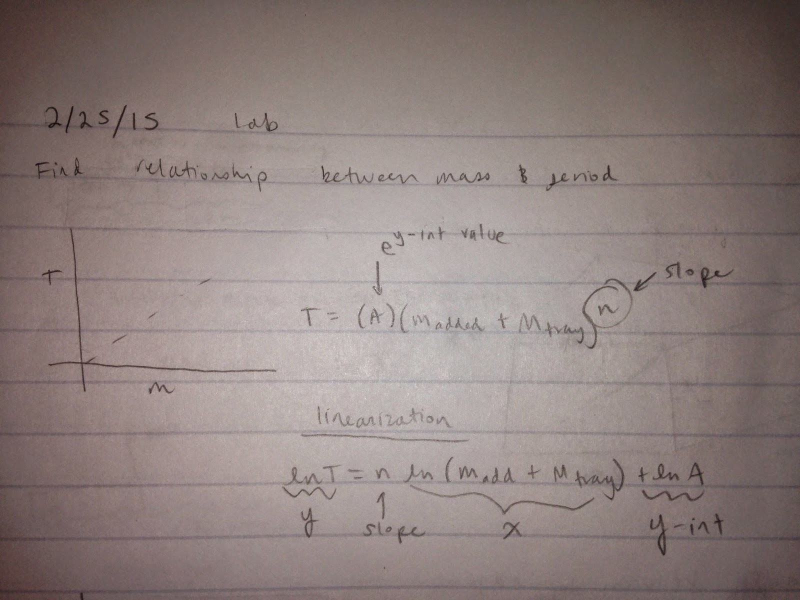
To find the relationship between mass and period, we guessed that period is related to mass by a power law type of equation T=A(m+Mtray)^n

Our first step was to record the period with no mass on the inertial balance, then record the period for every 100 grams added until reaching 800 grams. This measured data would help us solve for three unknowns A, Mtray, and n. By taking the natural logarithm on both sides of the power law equation we derived an equation very similar to y=mx+b. We plotted a graph of T vs. ln(m+Mtray) and created a parameter of what our mass of the tray should be in order to get a nice straight line and correlation coefficient value close to 1. To determine the mass of the two unknowns we needed a range of Mtray, which included a maximum and minimum value. These values were .280 kg (min) and .362 kg (max). By examining the slope and y-intercept of these two values, we were able to determine the values of A and n and model an equation to give us a range of masses for our unknowns.

Data Table

Screen Shot of T vs. ln(m+Mtray)

Minimum value for Mtray

The minimum value for Mtray was .280 kg. This yielded fit parameters of n= 0.6509 and a y-int= -0.4169

Maximum Value for Mtray

The maximum range value for Mtray was .362 kg. This yielded fit parameters of n= .07499 and a y-int= -0.4703

The main purpose of finding a range of mass values was because there is some uncertainty in our modeled equation and having a range, each value of Mtray would have its own y-intercept and slope value to give us sufficient curve fits. 

Derivation of Modeled equations

     

  

        Range of calculated mass values    

  

Unknowns

Water Bottle

Period .566600 s

Max value .515 kg

Min value .512 kg

Actual mass .469 kg

Tape Roll

Period .370272 s

Max value .136 kg

Min value .132 kg

Actual mass .125 kg

In this lab, an inertial balance was set up to find the relationship between mass and period. The periods of various known masses were used in order to model an equation so that we could find the unknown mass of two objects and compare them with a measured scale mass. A minimum and maximum value for Mtray were recorded along with its parameters, which both needed a correlation coefficient as close to the value of 1 as possible, in order to give us a somewhat accurate range of mass for our two unknowns. Unfortunately, our modeled equation did not yield good results. Our calculated mass and measured mass were somewhat off. This could have been due to various reasons such as the uncertainty of our equation and what we ignored such as placement of mass on the inertial balance and the amount of tape used to hold down our unknowns could have deviated the actual period the photogate measured.